Fused mxfp4 quantization & matmul kernel on the AMD MI355X

Bits	Kind	Value
`S'00'0`	zero	$\pm 0$
`S'00'1`	subnormal	$\pm 0.5$
`S'01'0`	normal	$\pm 1$
`S'01'1`	normal	$\pm 1.5$
`S'10'0`	normal	$\pm 2$
`S'10'1`	normal	$\pm 3$
`S'11'0`	normal	$\pm 4$
`S'11'1`	normal	$\pm 6$

Matrix multiplication

Now that we have an efficient quantization routine, let’s take a closer look at the matrix multiplication itself. In particular, we will use matrix cores (AMD’s answer to NVIDIA’s tensor cores) to accelerate the tiled computation.

An important part is that the input shapes are fixed, which will allow us to come up with specialized approaches later.

M	N	K
4	2880	512
16	2112	7168
32	4096	512
32	2880	512
64	7168	2048
256	3072	1536

The small M sizes, relative to the other dimensions, call for dedicated approaches in particular, as we will see later.

Matrix core layouts

The input B matrix is already given in mxfp4 format, so we naturally want to use the MI355X’s support for low-precision datatypes. In particular, two instructions are available: v_mfma_scale_f32_16x16x128_f8f6f4 and v_mfma_scale_f32_32x32x64_f8f6f4. The host code strongly steers us toward the former, because it shuffles the B weights in $16$ -row blocks to match that instruction’s hardware register layout.

MFMA operations require wave-level cooperation: each lane holds its share of the A, B, and C weights, along with the corresponding scales. The exact layout is specified in the CDNA4 ISA manual.You can find it here. The layouts for v_mfma_scale_f32_16x16x128_f8f6f4 are in sections “7.1.5.1. Dense Matrix Layouts: 8-bit and Smaller” for the weights, and “7.2.1. MFMA with Block Exponent Scaling” for the scales.

The input A and B matrices are laid out column-major with respect to the lane index. Each lane holds 32 values (one mxfp4 block), packed into four 32-bit registers, corresponding to 32 columns along the K dimension.

Weights/scales register layout for the A/B input matrices, with v_mfma_scale_f32_16x16x128_f8f6f4

The host code shuffles the prequantized B matrix to match this layout. In effect, it breaks the matrix into $16\times 32$ subtiles,The python snippet uses 16-by-16, because PyTorch treats the data as fp4x2 (basically, addressing bytes), so that 16 elements are actually 32 fp4 values. then swaps the axes so that the weights within each 2D tile become contiguous in memory.
This shuffling lets us read an entire $16\times 128$ B tile with a single instruction (e.g. global_load_dwordx4).

B_swiz = (
    B_q.view(-1, 16, B_q.shape[1] // 16, 16)
        .permute(0, 2, 1, 3)
        .contiguous()
        .view(*B_q.shape)
)

The B scales are also shuffled, but with one extra complication: the host code packs them into a $2\times 2$ MFMA supertile (i.e. $32\times 256$ in total), so four consecutive e8m0 values actually belong to different tiles.

Bs_swiz = (
    Bs.view(-1, 2, 16, Bs.shape[1] // 8, 2, 4)
        .permute(0, 3, 5, 2, 4, 1)
        .contiguous()
        .view(*Bs.shape)
)

Below is a little visualization of this shuffling. The point is that, with a single load instruction, a wave can fetch the scales for four closely related tiles and perform eight MFMAs to produce an output supertile. This increases the arithmetic intensity of AITER’s matmul kernel, since it does more work for the same data movement. However, it also greatly complicates address calculations for code that does not follow the same scheme (as I found out the hard way).

On the other hand, the output/accumulation C matrix is laid out row-major, with each lane holding four fp32 values in four separate registers:

Weights register layout for the C output matrix, with v_mfma_scale_f32_16x16x128_f8f6f4

This discrepancy between input and output layouts is one of the quirks of AMD matrix cores. By contrast, NVIDIA builds its layouts from a $16\times 16$ “core matrix” (see fig. 3a in this paper).

A basic matmul kernel

Now that we understand the register layout and the input pre-shuffling, we have all the pieces in place to build a simple first matmul kernel.

To keep things simple, we will divide the output into $16\times 16$ tiles (the shape of the matrix core instruction), and assign a separate block to each one, consisting of a single full wavefront (64 threads). The kernel then walks the K dimension in steps of 128 (the size processed by each MFMA instruction), quantizes the A tile, accumulates the C tile into registers, then finally writes out the results to global memory.

Here is the kernel (check it on godbolt):

__global__ __launch_bounds__(64) __attribute__((amdgpu_waves_per_eu(2, 2)))
void kern_mm(bf16 *C_ptr, const bf16 *A_ptr, const fp4x32 *B_ptr, const fp8e8m0 *Bs_ptr, 
             u32 m, u32 n, u32 k) 
{
    // Inform the compiler about problem shapes (removes some pessimistic branches)
    __builtin_assume(m >= 4 && n >= 2112 && k >= 512 && (m & 3) == 0 && (k & 511) == 0);

    auto tid = threadIdx.x, lid = tid & 63;
    auto C_tile_x = blockIdx.x, C_tile_y = blockIdx.y,
        C_x = C_tile_x * mxc_tile_y, C_y = C_tile_y * mxc_tile_y;

    // Iterate through the K dimension
    fp32x4 C = {};
    for (u32 it = 0; it < k; it += mxc_tile_x) {
        auto *ptr = reinterpret_cast<const AliasedBlockBf16 *>(A_ptr + (C_y + (lid & 15)) * k + 
                                                               it + (lid >> 4) * 32);
        auto A = *ptr;

        // Hint the compiler to schedule the Bq loads after A, only allow
        // ALU instruction to move across this boundary
        __builtin_amdgcn_sched_barrier(1);

        auto Bq = alias(AliasedBlockFp4, B_ptr[(C_tile_x * k + it) / mxc_tile_x * 64 + lid]);

        auto Bs = Bs_ptr[(C_tile_x / 2 * k / mxc_tile_x / 2 + it / mxc_tile_x / 2) * 64 * 4 +
                         lid * 4 + ((it / mxc_tile_x & 1) * 2) + (C_tile_x & 1)];

        auto [Aq, As] = quantize_block_mxfp4(A);

        // The intrinsic requires 8 dwords for the A/B matrices, 
        // because it has to support the fp8 version,
        // but the compiler will eliminate unused top 4 dwords.
        C = __builtin_amdgcn_mfma_scale_f32_16x16x128_f8f6f4(
            u32x8{Aq.u32[0], Aq.u32[1], Aq.u32[2], Aq.u32[3]},
            u32x8{Bq.u32[0], Bq.u32[1], Bq.u32[2], Bq.u32[3]},
            C,
            4, 4,   // A/B dtype selection (fp4)
            0, As,  // A block scale opsel + value
            0, Bs); // B block scale opsel + value
    }

    // Write the C tile into global memory using nontemporal stores,
    // to avoid evicting useful data from the caches.
    if (C_y + (lid >> 4) * 4 < m) {
        for (u32 i = 0; i < 4; ++i)
            __builtin_nontemporal_store(static_cast<bf16>(C[i]),
                C_ptr + (C_y + (lid >> 4) * 4 + i) * n + C_x + (lid & 15));
    }
}

Already, a few things are worth noting:

Two compiler hints to improve codegen:
- One on the input constraints, which removes an early check on K to see whether it is non-zero (which is always true for our shapes).
- Another on the loading, to force it to separate A and B reads. This way, the code can wait on B/B-scales to arrive only after quantization is finished.
We use nontemporal stores on the output, since this data will not be reused and does not benefit from caching. It helps reduce cache pressure and keep useful data around.
We force the compiler to use vector registers (VGPRs) instead of accumulator registers (AGPRs) for the MFMA with -mllvm=--amdgpu-mfma-vgpr-form=1, which removes a few data movement instructions (v_accvgpr_{read,write}_b32). In my experience, this is redundant with the amdgpu_waves_per_eu attribute since LLVM will prioritize VGPRs when it knows only few waves will be resident (and thus it can use many VGPRs), but I prefer to make certain.

Block remapping and tile assignment

The MI355X has a stacked chiplet architecture, meaning that the card is made up of several chips fabricated separately, and later assembled into a single card. In particular, it separates compute and I/O dies: the former (XCDs) comprise the CUs and L2 cache, and the latter (IODs) hold the coherency units, L3 cache (aka. infinity cache), the memory controllers, etc. The 8 XCDs are physically bonded to the 2 IODs (4 XCDs per IOD) via a direct copper-to-copper process, and the two IODs are themselves placed on a passive silicon substrate that enables die-to-die communication through physical interfaces (PHYs).Check this paper for an excellent exploration of the fabrication/design processes involved.

The critical part is that each XCD has its own private L2 cache, so we want to make sure that blocks resident on the same XCD are operating on related data, to maximize reuse and minimize cache pressure. However, blocks are dispatched in a round-robin manner across XCDs, such that consecutive blocks are actually physically located on different compute (and even sometimes I/O) dies.
Thus, we want to “remap” the block ID so that consecutive blocks end up on the same XCD.

Compute and I/O chiplet configuration for the MI355X, and vanilla/remapped block IDs for a 24-wide dispatch

Basically, what we want to do is move the 3 LSBs of the block ID, which represent the XCD ID, to become the MSBs of the remapped block ID (so essentially, a 3-bit right-rotate). For a variable grid size gsz, the remapped block ID rbid can be calculated from the original bid with this expression:

rbid = (bid & 7) * (gsz >> 3) + (bid >> 3);

On top of that, we want to assign spatially nearby output tiles to blocks on the same XCD. This way, the portions of the A and B matrices can be held in the L2 and reused across different CUs:

Tile assignment for improved cache reuse. Here we would assign 4 CUs on the same XCD to process tiles 0 to 3, and benefit from the reuse of rows/columns of A/B, respectively.

Since our input shapes are known and have a relatively small M, we can just assign consecutive blocks to the same column of the C matrix. The output tile indices can therefore be calculated from the remapped block index with:

C_tile_x = rbid / tm, C_tile_y = rbid % tm;

with tm the number of 16-high tiles in the C matrix (i.e. M / 16). In addition, since M is always a power of 2, we can optimize the expensive integer division and modulo operationsThe MI355X has no instruction-level support for these operations on integers, so it will convert back and forth between integers and fp32 (see godbolt, note the v_cvt_* conversion instructions). On the other hand, there is a CTZ instruction (v_ffbl_b32). with:

C_tile_x = rbid >> __builtin_ctz(tm), C_tile_y = rbid & (tm - 1);

Shuffling A through LDS

At this point, our access pattern for loading A is pretty inefficient: since we need each lane to hold a block of 32 weights, we are issuing 4 global_load_dwordx4 instructions. However, the addresses are disjoint, leading to poor coalescing and emitting more load requests than necessary. Instead, we would like to load 4 rows of the A tile per instruction, then shuffle the data into the correct locations.

For this, we can use LDS: the weights are first loaded to shared memory using coalesced accesses, then each lane reads the data it needs from fast local memory.
In particular, we use direct global-to-LDS loads, bypassing an intermediate step in registers. This is done via the buffer_load_dwordx4 instruction. The code looks like this:

// Build buffer descriptor for A
// We disable exceptions (user_vm_mode = 0), since the code will issue OOB loads for M < 16
auto A_rsrc = __builtin_amdgcn_make_buffer_rsrc(reinterpret_cast<void *>(A_ptr), 0, m * k * sizeof(*A_ptr), 0x10000);

// LDS storage for a single A tile, used for loading/shuffling into VGPRs
__shared__ AliasedBlockBf16 A_lds[mxc_tile_x*mxc_tile_y/mxc_qblock_sz];

for (u32 it = 0; it < k; it += mxc_tile_x) {
    // Load A tile into LDS
    // We need (128*16*2) / (64*16) = 4 requests per tile, each loading 4 rows in the M dimension
    auto A_voff = (lid >> 4) * k + (lid & 15) * 8,
         A_soff = C_y * k + it,
         A_incr = 4 * k;
        
    for (u32 i = 0; i < 4; ++i) {
        __builtin_amdgcn_raw_ptr_buffer_load_lds(
            A_rsrc,
            static_cast<void *>(A_lds + i * 16),
            16,                                                     // Load size
            static_cast<u32>( A_voff               * sizeof(bf16)), // Global offset (via VGPR)
            static_cast<u32>((A_soff + i * A_incr) * sizeof(bf16)), // Global offset (via SGPR)
            0,                                                      // Global offset (via immediate)
            0);                                                     // Cache policy flags
    }

    // Load B/B-scale...

    // Shuffle A from LDS into registers
    auto A = A_lds[(lid & 15) * 4 + (lid >> 4)];

    // Quantize A + perform MFMA...
}

// Epilogue...

One small optimization is achieved via the buffer descriptor: we instruct the hardware to not emit faults when accessing out-of-bounds data, and instead return zeroes. This is useful when M is smaller than 16: we can remove a bounds check in the loading code, and the invalid requests will “complete” immediately, additionally clearing the uninitialized LDS.

Resolving bank conflicts with swizzling

The code above has an issue: it accesses LDS with a stride of 64B (32 bf16 elements) during the readout of A from LDS.It might not look like it from the code but keep in mind the size of each AliasedBlockBf16 is 64B, and the compiler has to break down the load into 4 ds_read_b128 instructions, hence the bank conflict issue. This is problematic, because it creates LDS bank conflicts.

The LDS block on the MI355X is made up of 64 independent banks each containing 640 dwords (i.e. 160 KiB in total). Additionally, LDS accesses are performed in phases: if more than one address maps to the same bank during the same phase, then the accesses must be serialized, hence creating a conflict and requiring additional time to complete.

The phase pattern for ds_read_b128 is documented here. If we superimpose it with our LDS layout for the A tile, the bank conflicts become obvious:

LDS layout for the A tile in bf16 format, without swizzling

In the figure above, each square represents a bank element (32 bits), which contains 2 bf16 values. The MFMA tile K-size (128 bf16) matches perfectly the number of banks, such that one row of the A tile engages all 64 banks. This also means that each column of the tile is stored in the same bank. 4 ds_read_b128 instructions are necessary to complete the load from LDS, each reading 16 columns.
The problem arises because lanes try to read columns of A: we have an 8-way bank conflict, as 8 lanes per phase try to access the same bank.

Since we have the same number of lanes and banks (64), we must somehow spread out the accesses so that one bank is activated exactly once per phase. At the same time, we need to keep groups of 8 bf16 elements consecutive (i.e. 16 bytes), because of the MFMA register layout. Therefore, the lowest $\log_2(16)=4$ bits of the LDS load address will remain untouched.

Looking again at the phase pattern, we notice the accesses are done in “squares” of $4\times 4$ , so the first step is to make these squares access different banks. To achieve this, we need to modify the $\log_2(4)=2$ bits after the 4 LSBs, i.e. the 4th and 5th. We would like them to change values when reaching another row, which is controlled by the $\log_2(64*4)=8$ th bit onwards. So putting this together, we need to XOR the 4th and 5th bits with the 8th and 9th: swizzled = ((addr >> 4) & (0b11 << 4)) ^ addr.

This doesn’t fix everything, though: pairs of “squares” are still accessing the same banks. We have improved to a 2-way bank conflict, but there is still one step to go. Currently we are engaging banks 0-15 and 16-31 (each twice per phase), so we need to get banks 32-63 into the mix. Following the same reasoning as before, we switch the value of the $\log_2(32*4)=7$ th bit when we reach another group of 4 rows, i.e. when the $\log_2(64*4*4)=10$ th bit is activated. With this, the final swizzling expression becomes:

auto swiz = [](u32 addr) {
    return (((addr >> 4) & (0b11 << 4)) | ((addr >> 3) & (0b1 << 7))) ^ addr;
};

The swizzled LDS layout looks like this:

LDS layout for the A tile in bf16 format, with swizzling

Notice how phases access each bank exactly once. Since XOR is involutive (i.e. A ^ B ^ A = B), and the transform does not modify bits which are later used as input, we can use this same swizzling pattern when loading into LDS and reading results back to registers.

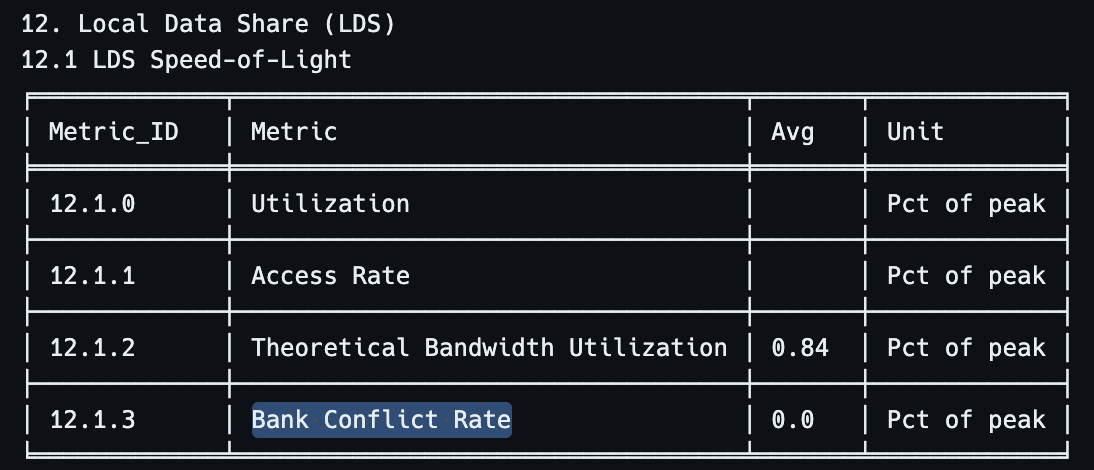
To make sure bank conflicts are fixed, we can check in rocprof-compute:

Bank conflict rate in the kernel, after swizzling

Double-buffering

With the addition of global-to-LDS loads, we are just one step away from achieving better compute/memory overlap. Indeed, at the moment we are processing these two operations serially: a wave first loads A/B tile data, then performs quantization and MFMA. For the entire duration of the load, the wave is idling, as can be seen in the trace below.

⊕ Show captionFigure 10: Hardware trace of a loading/compute phase with serial loading

The idea of double buffering is simple: using LDS as a staging buffer, we initially perform a load operation (i.e. load an A/B tile pair), then ping-pong between load and compute until completion. Since the compute operation processes data that was loaded in the previous phase, it overlaps with the next load. Essentially, we are pipelining loading and compute.
In code, it looks like this:

// LDS staging buffers
__shared__ bf16x8  A_lds [2][mxc_tile_x*mxc_tile_y/8];
__shared__ fp4x32  Bq_lds[2][mxc_tile_x*mxc_tile_y/32];
__shared__ fp8e8m0 Bs_lds[2][mxc_tile_x*mxc_tile_y/32*4];

auto load_to_lds = [&](u32 it, u32 phase) __attribute__((always_inline)) {
    // Issue buffer loads for A weights, and B weights/scales...
};

auto do_compute = [&]<int outstanding>(fp32x4 &C_dat, u32 it, u32 prev_phase, C<outstanding>) __attribute__((always_inline)) {
    __builtin_amdgcn_s_waitcnt(0xf70 | outstanding);

    // Read A from LDS, quantize to mxfp4
    auto A_dat = AliasedBlockBf16{};
    for (u32 i = 0; i < 4; ++i) {
        auto idx = ((lid & 15) * 4 + (lid >> 4)) * 4 + i;
        A_dat.x8[i] = A_lds[prev_phase][idx ^ swiz(idx)];
    }

    auto [Aq_dat, As] = quantize_block_mxfp4(A_dat);

    __builtin_amdgcn_s_waitcnt(0xf70 | (outstanding - 2));

    // Read B weights/scales from LDS
    auto Bs_dat = reinterpret_cast<u32 *>(Bs_lds[prev_phase])[lid];
    Bs_dat >>= ((C_tile_x & 1) + (it / mxc_tile_x & 1) * 2) * 8;

    auto Bq_dat = alias(AliasedBlockFp4, Bq_lds[prev_phase][lid]);

    // Accumulate
    C_dat = __builtin_amdgcn_mfma_scale_f32_16x16x128_f8f6f4(
        u32x8{Aq_dat.u32[0], Aq_dat.u32[1], Aq_dat.u32[2], Aq_dat.u32[3]},
        u32x8{Bq_dat.u32[0], Bq_dat.u32[1], Bq_dat.u32[2], Bq_dat.u32[3]},
        C_dat, 4, 4, 0, As, 0, Bs_dat);
};

// Initial loading phase
u32 it = 0, prev_it = it, phase = 0, prev_phase = phase;
load_to_lds(it, phase);

fp32x4 C_dat = {};
for (it = mxc_tile_x, phase = 1; it < k; prev_it = it, it += mxc_tile_x, prev_phase = phase, phase ^= 1) {
    load_to_lds(it, phase);
    do_compute(C_dat, prev_it, prev_phase, C8);
}

// Final compute phase
do_compute(C_dat, prev_it, prev_phase, C2);

// Write C tile to global memory...

With tracing, we can see how much the idling has been reduced:

⊕ Show captionFigure 11: Hardware trace of a loading/compute phase with pipelined loading

One difficulty with this pattern is that the compiler does not attempt to keep track of dependencies on data loaded directly to LDS, so we need to guard it ourselves. This is achieved via the s_waitcnt instruction, which makes the waves wait until the vmcnt (vector memory count) counter has reached a specific value.On AMD GPUs, all memory operations are asynchronous. When a wave issues a memory instruction, a counter is incremented, that will be decremented when the request completes (note that operations are reported in-order). There are different counters for global memory (vmcnt) and LDS (lgkmcnt). The lgkmcnt counter is also used for other things, but this is not relevant here. Since we know each wave issues 6 buffer_load instructions (4 for A, 1 for B weights and 1 for B scales), and we have two loading phases in-flight in the hot loop, we guard A until vmcnt reaches $6\times 2-4=8$ , and B/B-scales with $6\times 2-4-2=6$ . In the last compute phase, only one loading operation is pending, so the counter thresholds become 2 and 0, respectively.

Blocked kernel variant

Our not-so-basic-anymore kernel is now in pretty good shape. However, the core of the approach remains fairly naive: we are dispatching one block per output tile, regardless of the input shapes. In some cases, it might be beneficial to increase the block size and de-duplicate some quantization calculations by sharing results between waves via LDS. This is especially true for the last two shapes (M/N/K 64/7168/2048 and 256/3072/1536).
Processing multiple tiles per block also fits the B-scale shuffling better, and simplifies address calculation.

The blocked kernel launches 4 waves per block (i.e. 256 threads in total). Just like in the previous kernel, each wave is assigned a single $16\times 16$ output tile of C. Together, the block manages a $32\times 32$ portion of C, which allows waves to share quantization results.
Each wave therefore does 2 MFMAs per phase instead of 1:

Overall, the code is very similar to the basic version, with the addition of extra LDS handling to share/retrieve quantized A values (no swizzling is needed here).

If we look at the MFMA operations, we can see that each wave will use its own quantization results at some point (i.e. wave 0 will use A0, wave 1 will use A1, etc.), meaning we can avoid having to wait for the associated LDS store/load and just use data that’s already in registers.

Considering now the B-scales, we’ve seen before how they are shuffled so that each contiguous 4 bytes contain scales for a $2\times 2$ MFMA super-tile. In order, waves 0/2 will need scales for tiles 0/1, and waves 1/3 scales for tiles 3/2. This reversal makes things a bit awkward, I solved it by using the v_perm_b32 instruction, which allows reordering bytes within a 32-bit word.This instruction is a carry-over from back when GPUs were actually designed for graphics, because a common shader programming pattern is to “swizzle” color components (in GLSL, this looks like col.bgra for instance). The permute pattern does two things at once: swap the 3rd and 4th values, and switch from N-major ordering to K-major.
After that, waves will select the correct value pair, and pass the scale to the MFMA instruction. The first MFMA uses the value at byte position 0, and the second MFMA the one at position 1, which is possible via the opsel field.

// Read B scales for the 2x2 super-tile, permute and discard
auto Bs_dat = reinterpret_cast<u32 *>(Bs_lds[prev_phase])[lid];
Bs_dat = __builtin_amdgcn_perm(Bs_dat, Bs_dat, 0x01030200) >> ((wid & 1) * 16);

// Other setup code...

// First MFMA, use first byte of packed B-scale value
C_dat = __builtin_amdgcn_mfma_scale_f32_16x16x128_f8f6f4(..., 0, Bs_dat);

// Second MFMA, use second byte of packed B-scale value
C_dat = __builtin_amdgcn_mfma_scale_f32_16x16x128_f8f6f4(..., 1, Bs_dat);

You can check the complete code for this kernel on godbolt. Hardware tracing shows a much tighter hardware utilization, with fairly little stalling:

Split-K kernel variant

There remains a problematic input shape: M=16, N=2112, K=7168. In this case, we don’t even have enough output tiles (132) to properly occupy the whole GPU (256 CUs), and K is quite long (56 MFMAs), leading to a very long accumulation loop. One way to address this is to use a split-K method: waves process only a portion of the K dimension, and combine their results just before output.
This sharding lets us reach much higher parallelism.

You can check the complete code for this kernel on godbolt.

Other optimizations

Kernarg preloading

At entry, the kernel must load its arguments (data pointers and shapes). This reads from the “kernarg” segment, which is commonly located in host memory.This location is chosen to avoid having to invalidate the L2 cache at kernel boundaries, because host-mapped memory is uncached. The result is one unavoidable, uncached load that takes about 1000 cycles, i.e. ~0.4 µs at the MI355X peak clock of 2400 MHz (see the trace below).

⊕ Show captionFigure 15: Hardware trace during kernarg loading

Instead, we can instruct the hardware to preload some of that data into SGPRs before the CUs start executing (see here). This is controlled by the -mllvm=--amdgpu-kernarg-preload-count=N compiler flag (where N is the maximum number of arguments to preload, not the number of dwords).
Execution then begins at entry+0x100, which lets LLVM insert a trampoline in case the hardware does not support preloading (you can inspect this on godbolt).

After applying this change, the waiting time is much shorter:

Why wasn’t it eliminated entirely? The reason is that the hardware limit for preloading is 16 registers.This is documented in the ISA manual, section 3.13 “GPR Initialization”. That should have been enough for us, except that the compiler also enables the kernarg segment pointer in SGPRs 0/1 for the trampoline, effectively reducing the useful capacity to 14 dwords. That pushes the final argument over the limit, which means we still need a single s_load_dword.
This issue only appeared several iterations after enabling kernarg preloading, once a few more kernel arguments had been added, so I didn’t notice it at the time. Fortunately, it can likely be fixed with some small argument type adjustments.

Dynamic wave priority

When a wave switches to a loading phase, we want it to issue its load instructions as quickly as possible to minimize latency. Since several waves can be resident on a single SIMD core, we may run into slowdowns if the CU decides to schedule other work first. One possible solution is to raise the wave’s runtime priority during the loading phase, using the s_setprio instruction. Before returning to the compute phase, the priority is reset to its baseline value.

auto load_to_lds = [&](u32 it, u32 phase) __attribute__((always_inline)) {
    __builtin_amdgcn_s_setprio(1);

    // Load tiles...
};

auto do_compute = [&]<int outstanding>(fp32x4 &C_dat, u32 it, u32 prev_phase, C<outstanding>) __attribute__((always_inline)) {
    __builtin_amdgcn_s_setprio(0);

    // Quantize/accumulate...
};

This didn’t produce a noticeable improvement, probably because there wasn’t any real execution-side congestion to begin with, but I still believe the underlying idea is sound.

Output shuffling

The output path currently issues four separate store instructions (each writing 2 bytes per lane) because of the matrix-core layout of the C matrix. With LDS, we can reduce that to a single store of 8 bytes per lane.

Since the elements of C are arranged column-major within each lane’s registers, a naive approach would require five LDS instructions (either one store plus four reads, or four stores plus one read) to transpose them. However, the MI355X has a special LDS read instruction, ds_read_b64_tr_b16, that can transpose the result of an LDS read. The exact transpose pattern is not clearly documented, but after some testing I found it equivalent to the following permutation for a $16\times 16$ matrix of bf16 elements:

tr = (
    torch.arange(64*4, dtype=torch.bfloat16)
        .reshape(-1, 4, 4, 4)
        .permute(0, 2, 3, 1)
        .reshape(16, 16)
)

Or, in diagram form:

Shuffling performed by ds_read_b64_tr_b16 on a 16\times 16 matrix of bf16 elements

Using this method, we can transpose C with only two LDS instructions: one store and one read.

__shared__ bf16x4 C_lds[mxc_tile_y*mxc_tile_y/4];

// Transpose the C tile to row-major using LDS
// Each lane holds 4 (fp32) values of a column of C, ds_read_tr16 allows switching to row-major.
// With some shuffling on top of that, we can issue a single global_store_dwordx2 instead of 4,
// which will be coalesced in the TA unit regardless of the shuffling.
// ds_read_tr16 requires all lanes to be active, so do the shuffling outside of the if-guard.
auto shfl = ((lid & 3) << 2) + ((lid >> 2) & 3) + (lid & ~15);
C_lds[shfl] = bf16x4{ static_cast<bf16>(C_dat[0]), static_cast<bf16>(C_dat[1]),
                      static_cast<bf16>(C_dat[2]), static_cast<bf16>(C_dat[3]), };

// No barrier needed here since we have only one wave executing
auto res = __builtin_amdgcn_ds_read_tr16_b64_v4bf16((__attribute__((address_space(3))) bf16x4 *)C_lds + lid);

// Write the C tile into global memory using a nontemporal store,
// to avoid evicting useful data from the caches.
if (C_y + (lid >> 4) * 4 < m) {
    __builtin_nontemporal_store(res,
        reinterpret_cast<bf16x4 *>(C_ptr + (C_y + (shfl >> 2)) * n + C_x + ((shfl & 3) << 2)));
}

Unfortunately, this does not produce a noticeable improvement in kernel runtime. The original idea was to use it in the blocked kernel, since it would allow stores for horizontally adjacent tile pairs to be coalesced and could potentially speed up the epilogue. On AMD GPUs, kernels terminate by issuing the s_endpgm instruction, which implies waiting for all outstanding memory operations to complete (see the trace below). By reducing the number of in-flight store requests, we could potentially shave off some of that latency.
However, I ran out of time to implement this change.

Execution tail due to waiting on stores to complete

Fused mxfp4 quantization & matmul kernel on the AMD MI355X

Introduction

Quantization

The mxfp4 format

Hardware-assisted quantization

Finding the block magnitude

Calculating the scale

Matrix multiplication

Matrix core layouts

A basic matmul kernel

Block remapping and tile assignment

Shuffling A through LDS

Resolving bank conflicts with swizzling

Double-buffering

Blocked kernel variant

Split-K kernel variant

Other optimizations

Kernarg preloading

Dynamic wave priority

Output shuffling

What was missing?

Host-side optimizations

Tighter memory loading

Loading everything upfront

Triple buffering

(Over-)specialization

Conclusion