Vulkan ProRes decoder: prologue

Introduction

This year I enrolled in Google Summer of Code for the FFmpeg project, mentored by Lynne (with hassn as backup), and working on a Vulkan shader-based decoder for Apple ProRes codec (profiles 4444 and 4444 XQ).
What does this mean? Let’s go over each of these terms:

• Google Summer of Code (henceforth GSoC) is an initiative by Google to promote open source (OSS) development via funding something resembling summer internships, within large OSS projects. “Students” are assigned “mentors” (usually prominent maintainers of these projects), and work on a task with a set of deliverables. In my case, this will last roughly 4 months starting in May 2025.
  Besides the actual task, students are also required to write two reports (one midway and one final), of which this post is part.
• FFmpeg is a solution for media de- and en-coding, filtering, scaling, etc. It’s one of these projects that were founded by Fabrice Bellard before evolving into something ubiquitous: nowadays, FFmpeg powers most of the media world, from your browser to transcoding pipelines of cloud providers.
  The codebase is mostly made up of libraries (eg. libavcodec, libavfilter, libavutil), which provide different functionalities. The ffmpeg, ffprobe, etc. binaries then use these libraries to expose a command-line interface for them.
• Video work (capture, playback, …) has very high bandwidth requirements, due to the sheer amount of data that must be processed.On the order of 1 GB/s for even a 1080p stream at 24 Hz. In order to alleviate this, and take advantage of redundancies within the stream, standards have been developed, specifying an encoding scheme and the corresponding decoding operation. These are called “codecs”.
  Today, the most popular codec remains the trusty H.264, released in the early 2000s. H.264 is able to take advantage of spatial and temporal similarities, while also removing “details” in the video frames,Technically, spatial frequencies. This is achieved by converting a small area of the picture from spatial domain to the frequency domain, by applying a Fourier-like transform. Afterwards, the resulting coefficients are scaled down, and the smallest are culled depending on encoding parameters. which typically provides compression ratios of several orders of magnitude compared to the original stream. It is termed “lossy”, because the decoded data is different from the original stream.
• Apple ProRes is a codec developed by Apple, designed to provide visually lossless compression for tasks with high quality constraints, as well as good decoding performance. It is typically used during recording and editing of media, before the data is finally converted to another codec more suited to consumers. This is termed an “intermediate” or “mezzanine” codec.
  ProRes is not officially standardised, and used to be completely undocumented.In fact, the original commit adding reverse-engineered decoding support in FFmpeg was signed off under the pseudonym of Elvis Presley, due to legal risks. In 2015, Apple published an SMPTE disclusure document detailing the decoding process. While this technically doesn’t constitute a standard, it still provides an excellent overview of the codec features and decoding routines.
  ProRes contains different profiles with varying characteristics. In this work, we will focus on the 4444 and 4444 XQ profiles.
• Vulkan is a low-level graphics API, initially released in 2016 and designed to be cross-platform and low-overhead. It was thought up as a successor to OpenGL, whose design was becoming increasingly remote from the GPU hardware it was papering over.
  In Vulkan, GPU commands can be recorded and submitted from different threads, and hardware features are exposed without much abstractionThis is debatable. In reality, due to hardware differences that are sometimes hard to reconciliate, some features might be quite remote from the actual hardware behavior. An example of this is VK_EXT_shader_object, which maps almost perfectly to NVIDIA hardware, but is pretty hard to implement for other vendors. or delay with respect to the chip release.
  Vulkan programs can achieve higher performance than OpenGL by carefully managing resources, building and reusing command buffers from multiple threads, and using newer hardware features. The downside is that much of the complexity is moved from the driver to the application.
  Vulkan support is provided natively on most modern platforms, with the exception of Apple devices, and is nowadays fairly mature.

Now that the context is clearer, let’s move on with the rest of the introduction.

Motivation

Nowadays, consumer media resolutions and framerates have ballooned, reaching 8K (8192x8192 px) and several hundreds of Hz. This becomes problematic for even simple codecs such as ProRes, because of the huge computational and bandwidth requirements associated with processing this much data.
Meanwhile, graphics processing devices (GPUs) have quickly become one of the most important computing peripherals (especially since the AI craze), and are especially well suited to media processing, due to their parallel programming model. While CPUs are optimised for latency-critical logic tasks, GPUs excel at bandwidth-heavy arithmetic work.
A ProRes GPU-based decoderThis is different from traditional GPU-accelerated (often called hardware-accelerated) video decoding, exposed for instance by DXVA or VAAPI, where the device relies on dedicated silicon (an ASIC) designed for a specific codec, and separate from the main shader cores. Here, we use these programmable shading units to implement our decoder. is therefore desirable, particularly to speed up video editing software. In order to take advantage of modern GPU features and maximise cross-platform compatibility, we will use the low-level Vulkan API.

Apple ProRes overview

In this section, I will outline the principle of operation of the ProRes codec, focusing mostly on the relevant profiles (4444 and 4444 XQ). Most of the information here can be found within the aforementioned SMPTE document.

ProRes is an intra-codec, meaning each frame is encoded independently from the others. This is great for video editing, because when jumping around the video only a frame’s worth of data will be required, without needing to process keyframes first. However, this means it doesn’t take advantage of the temporal redundancies within the video stream, from which a large part of the compression originates in inter-codecs.
It supports up to 8k resolution, 4:4:4 subsampling (meaning the chroma planes are not downscaled compared to the luma data), up to 12 bits of depth for luma and chroma, and an optional alpha plane with up to 16 bits of depth.

Stream structure

A ProRes stream is constituted of several elements, or syntax structures, organised in a hierarchy:

• Frame header: one of the design goals of ProRes is fast random access, meaning that when seeking somewhere in the stream, there is little information to gather before decoding the actual frame. I’ve already mentioned how ProRes doesn’t do inter-prediction at all, but another consequence of this aim is that each frame must include all relevant metadata (dimensions, encoding parameters, color information, …).This is in contrast to H.264 or H.265, which try to minimise the amount of metadata sent during playback, by making frames inherit properties from a formerly signaled parameter set. This is packed into a frame header, which precedes the rest of the data.You may note that the ProRes stream doesn’t contain any frame timing information. This is left entirely to the container layer (eg. MXF).
• Picture header: a ProRes frame is divided into slices, which are essentially independent compression contexts. This helps with parallelism, because each of them can be decoded separately. The picture header contains information regarding the slice structure, including a slice table containing the offsets of the slices within the compressed bitstream.This is kept separate from the frame header for mostly historical reasons, as earlier ProRes profiles supported interlacing, in which a frame is made up of two interleaved, half-sized pictures (also called fields).
• Slice header: each slice includes its own slice header, informing the decoder of the compressed size of the luma and chroma plane, as well as a compression coefficient (the rescaling factor). Each slice contains a number of macroblocks (MB), which are 16x16 pixels large. Each MB is broken down further into 8x8 blocks. In 4:4:4 subsampling mode, a macroblock thus contains 4 luma and 4 chroma blocks. In addition, a picture can contain an optional alpha plane. If enabled, the alpha data will be packed after the color blocks (using a different compression scheme).

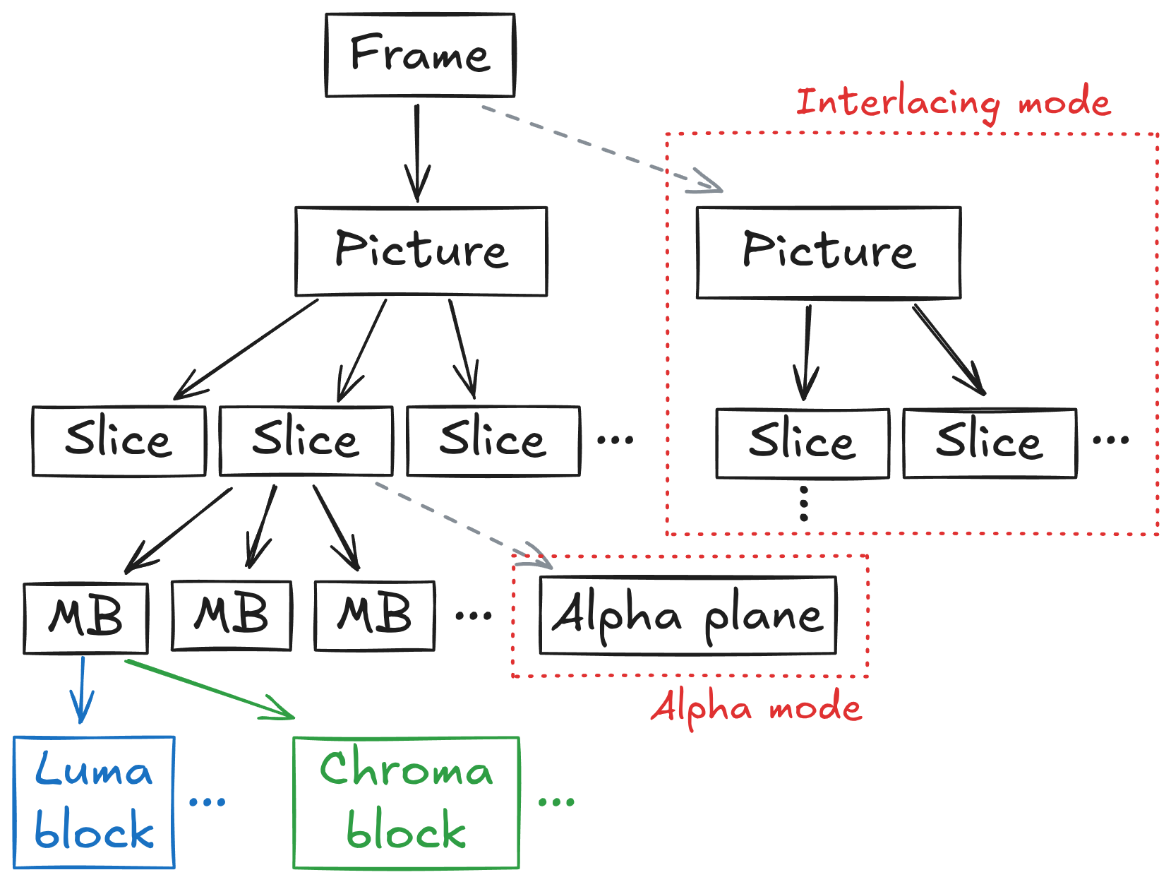⊕ Show captionFigure 1: ProRes structure hierarchy

Picture structure

A ProRes picture is broken down into slices which can be decoded in parallel, and contain a variable number of 16x16 MBs (up to 8). To this end, the stream specifies a parameter in the picture header, log2_desired_slice_size_in_mb. The picture data is then tiled into slices of this size, starting from the left. If the picture dimensions don’t exactly line up with the slice size, the remaining data is broken down in slices of the largest power of two that still fits, and this process is repeated recursively until the entire picture is covered. If a picture dimension is not a multiple of 16, the encode will slightly overshoot the picture size, and the stream consumer will have to discard or ignore the data past the specified frame boundary.

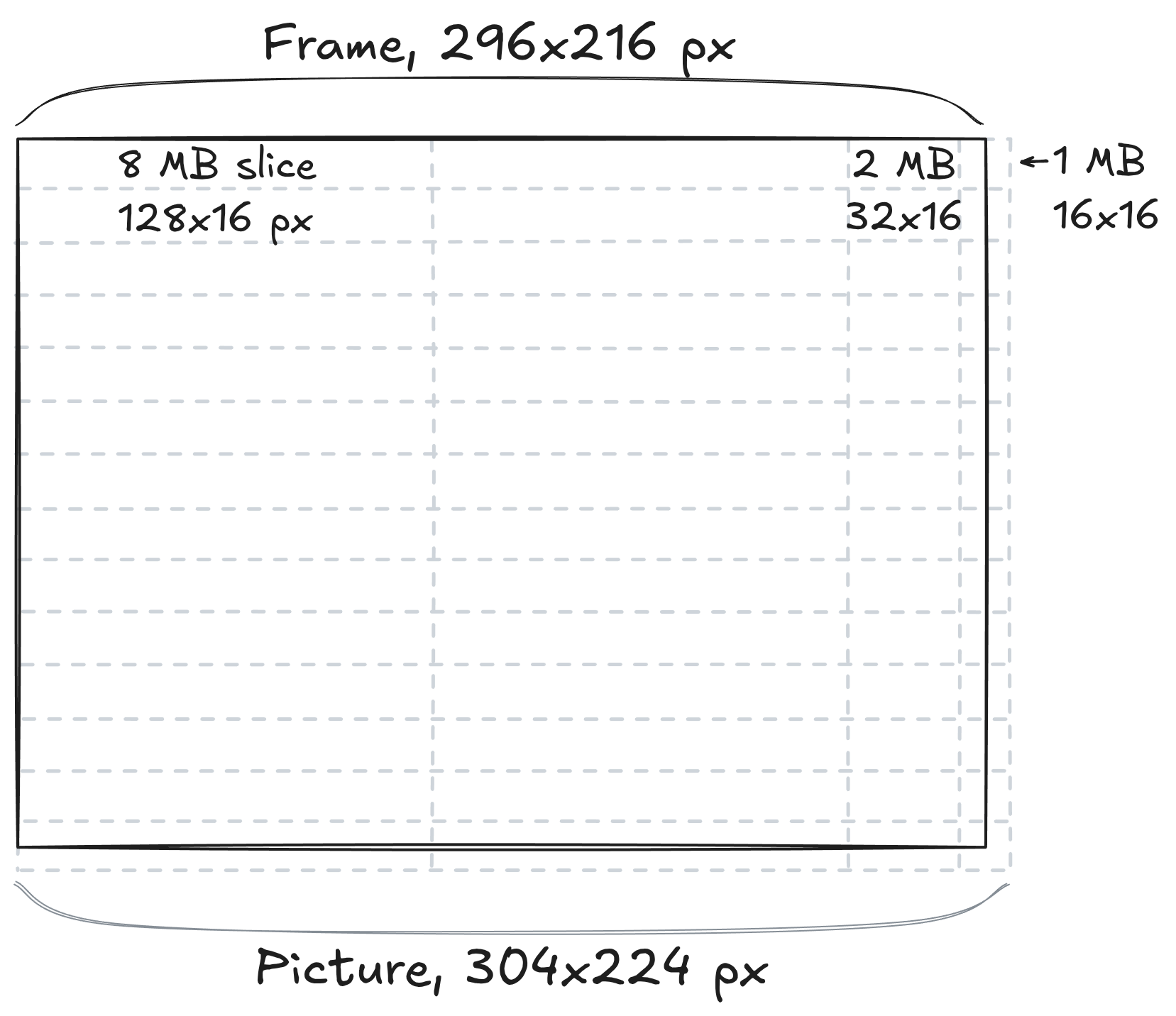⊕ Show captionFigure 2: ProRes frame structure.
The frame width is 296 px, which is not a multiple of 16 ($296 \bmod 16 = 8$). Since the frame header signals log2_desired_slice_size_in_mb = 3, the frame is first tiled by 2 slices of 128 px ($\lfloor 296 / 128 \rfloor$). The closest power of two to the 40 px left ($296 \bmod 128$) is 32, therefore the next slice contains 2 MBs. The final remainder is 8 px, so the last slice contains a single MB and the total picture size overshoots by 8 px.
Similarly, the picture is tiled vertically into 14 slices ($\lceil 216 / 16 \rceil$), and contains 8 extraneous pixels.

Slices can contain 1, 2, 4 or 8 macroblocks, arranged horizontally (ie. 16x16, 32x16, 64x16, or 128x16 px). MBs are made up of 8x8 px blocks, whose number depends on the subsampling scheme: there are always 4 luma blocks, but the number of chroma blocks can be 2 (for 4:2:2), or 4 (for 4:4:4). The chroma blocks are “stretched” in the final composite image, to cover the same area as the luma.Note that this is not the job of the decoder, whose task is simply to reconstruct the raw data contained within a compressed bitstream. In our case, the profiles we care about use 4:4:4 subsampling, ie. no chroma downscaling.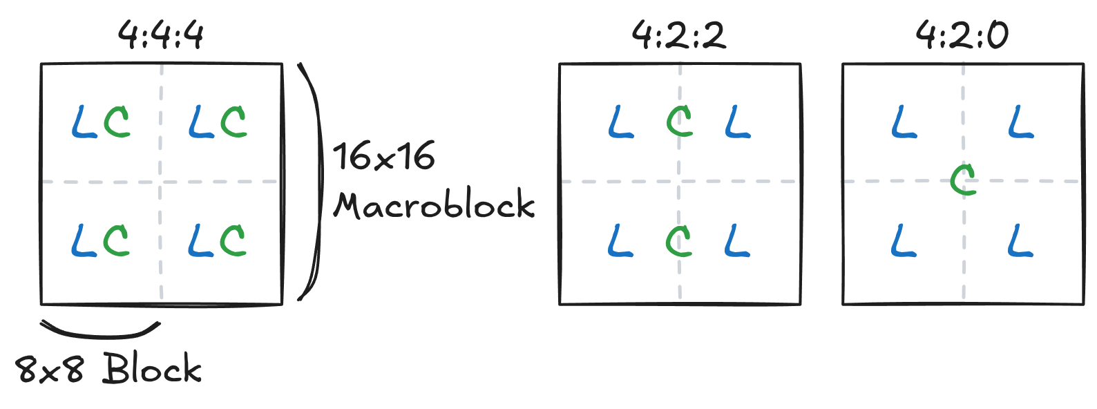

⊕ Show captionFigure 3: Luma and chroma sample locations for common subsampling schemes.
In 4:4:4 mode, each luma sample is associated a single chroma sample.
In 4:2:2 mode, each luma sample is associated 2x1 chroma samples (horizontal stretching).
In 4:2:0 mode, each luma sample is associated 2x2 chroma samples (horizontal and vertical stretching). Note that ProRes does not support 4:2:0.

Entropy coding

Entropy coding turns a sequence of fixed-width non-negative integers (the DCT coefficients) into a bitstream of variable-width codes.
ProRes uses a mix of the Golomb-Rice and exp-Golomb coding schemes, where small values are encoded with the former, and larger with the latter method.This favors decode speed, as the encoded DCT coefficients are mostly small in magnitude, and Golomb-Rice is computationally simpler than exp-Golomb. The scheme and the Rice/exp-Golomb threshold being used is determined according to the type of coefficient being encoded (DC/AC),The very first DCT coefficient (in the top-left corner of the transformed matrix) is often called “DC”, because it corresponds to a null frequency, and therefore represents a flat color over the whole spatial domain. Other coefficients are termed “AC”. its position within the bitstream (eg. whether it the first DC coefficient), and the magnitude of the coefficient that came before it.

Inverse scanning

The decoded coefficients have been packed in a way that increases entropy compression efficiency. The decoder must therefore rearrange them in the intended spatial order before proceeding.
The coefficients are placed in the stream essentially in a bottom-up direction with regards to the frame structure: each coefficient is grouped with its peers from other blocks, then other macroblocks. In addition, coefficients within blocks are scanned using a Morton curve pattern (illustrated in the 5th block in the figure below).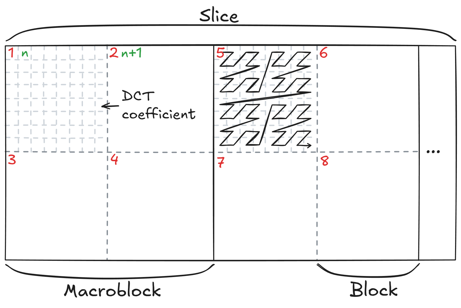

⊕ Show captionFigure 4: Scanning order
Red numbers indicate the first coefficients in the scanned stream, and their spatial position. Green numbers represent the second coefficients, and so on.

These reorderings result in a greatly increased locality and reduced entropy, by grouping together coefficients whose value is likely to be close. Indeed, spatial variations over the image tend to be small, and DCT coefficients typically have a decreasing magnitude when moving away from the top-left corner (the DC coefficient).The departure for zigzag scanning (used for instance in JPEG) is interesting, as zigzag more accurately represents the usual layout of DCT coefficients. This might be a tradeoff for decode speed, as a Morton order can be efficiently calculated using bitwise arithmetic, while zigzag ordering commonly requires a lookup table.

Scaling and transform

Reordering yields quantised coefficients $\mathbf{QF}$ organised in 8x8 frequency-domain blocks. Quantisation is the main source of compression in ProRes, and in effect is performed by a simple rounding division of the original matrix. To retrieve the de-quantised block, the inverse operation is performed, by multiplying with a global weight matrix $\mathbf{W}$. While the $\mathbf{W}$ matrix is global for the whole frame,While the weight matrix is global, it can be different for the luma and chroma components. It can also be set to the default one, in which case all its 64 components are 4. it is paired with a scalar, the rescaling factor $\mathit{qScale}$, which is signaled per-slice.
The rescaling operation is therefore: $\mathbf{F} = \mathbf{QF} \ast \mathbf{W} \ast \mathit{qScale}$.

The coefficients are then transformed from the frequency domain $\mathbf{F}$ to the spatial domain $\mathbf{S}$. This is achieved using the inverse discrete cosine transform (iDCT), with the expression given below.Note the similarity with the 2D Fourier transform. The sum range from 0 to 7 since the blocks are 8 px large, and produces a matrix of the same dimensions.While this operation (and in particular the nested sum) may seem intensive, there are clever ways of computing it rather efficiently.

with $C(n) = \begin{cases} 1/\sqrt{2} & \text{if \(n = 0\)}\\ 1 & \text{otherwise} \end{cases}$

After this operation, the decoding operation for luma and chroma components is essentially complete.There are a few steps remaining in order to calculate the final integer pixel data, and to output it at the correct location within the frame, but those are not particularly noteworthy.

Alpha plane

If present, the alpha data is encoded losslessly and without subsampling, in raster-scanned order.
The data is differentially encoded using RLE, meaning the difference of the current alpha value against the former gets encoded, and identical consecutive values are sent only once, along with the number of times they are repeated. For both the run lengths and the alpha delta, pre-defined tables are used to represent common small values using fewer bits.

State of the art

There is little software accelerating video decoding using GPU shaders, mostly due to the fact that most platforms already offer support for mainstream codecs such as H.264, H.265 or AV1, with dedicated hardware blocks.
A few proprietary solutions exist, such as the codec packs sold by MainConcept, or the decoders bundled with DaVinci Resolve.
In the open-source world, the most notable example is probably the FFmpeg project, which has been developing Vulkan-based acceleration for several codecs. There are also a few works towards JPEG, along with some relatively old academic exploration of this same codec.

FFmpeg Vulkan decoders

At the time of writing, FFmpeg includes a shader-based FFv1 decoder and encoder, and there has been some effort towards the VC-2 codec (as part of the 2024 GSoC event).
These codecs are however rather dissimilar to ProRes (FFv1 being lossless, and VC-2 based on the wavelet transform instead of DCT). However, the techniques used in entropy decoding could still be relevant for our work, and the shaders include some optimised variants making use of advanced hardware features (eg. subgroups).

JPEG decoders

The astute reader may have noted similarities between ProRes and JPEG.These similarities have led some to refer to ProRes as a “JPEG clone” (dixit #ffmpeg-devel). In particular, block sizes are the same, and the transform operation is identical (though JPEG quantisation lacks the $qScale$ parameter). Techniques employed by JPEG decoders can therefore be applied to some extent to our situation.

GPUJPEG

GPUJPEG is an open-source project developed by the Czech Educational and Research Network, and implements a JPEG codec in CUDA. It has some interesting optimisations especially regarding entropy decoding, though its implementation of the iDCT seems (from a cursory look) inferior to the one in the next project.

NVIDIA JPEG decoder

NVIDIA offers a JPEG decoder as part of their cuvid library. While cuvid is primarily meant to expose hardware codec functionality, NVIDIA chips lack, for the most part, a dedicated JPEG block.Recent NVIDIA GPUs (such as the A100 professional cards and Blackwell-generation consumer products) include such a purpose-built ASIC, called NVJPG. Tegra chips have also been bundling an NVJPG core for a long time. The library therefore uses a few CUDA programs to speed up decoding operations.
NVIDIA also provides CUDA sample showcasing the application of parallel programming to implement the (i)DCT, along with a whitepaper explaining the techniques used.

I’ve decided to reverse-engineer the CUDA binaries present in the cuvid library implementing this functionality. My goal here is two-fold: explore techniques used by NVIDIA developers themselves (who presumably have deep knowledge of parallel programming, along with access to internal documentation and tooling), and learn more about the low-level operation of NVIDIA shader cores, which should come in handy when optimising my own shaders.
However, this work is mostly unrelated to the present topic and this post is already running long, so I will be covering it in another blog post.

Conclusion

In this post, I exposed the motivation behind building a Vulkan-based ProRes accelerator within FFmpeg. I briefly overviewed the technical features and decoding process for this codec, which allowed me to solidify my knowledge.
In future posts, I will be referring to this text while exploring implementation details.